Un nuevo diseño de un sistema inteligente de administración de fármacos basado en partículas de nanoantenas

Resumen

El sistema de administración de fármacos de nanopartículas compuestas juega un papel importante en la interacción con los ganglios linfáticos. Hay tres tipos principales de linfocitos:células B, células T y células asesinas naturales. Cuando las células del sistema inmunológico se vuelven cancerígenas, atacan las células del cuerpo. El líquido linfático juega un papel importante en el ataque a las células sanas del cuerpo; por lo tanto, este artículo tenía como objetivo diseñar un sistema de administración de fármacos, que pueda dirigir eficientemente las nanopartículas para que apunten a las células infectadas, ayudando en la eliminación a alta velocidad de dichas células. El diseño propuesto depende de la interacción entre estas moléculas, y el nanocontrolador inteligente tiene la capacidad de guiar las nanopartículas por contacto anaeróbico. El diseño propuesto demostró que cuanto menor sea el tamaño y la densidad de las nanopartículas, menor será la viscosidad dinámica del líquido, lo que reflejaría su resistencia al flujo. Además, se concluyó que las moléculas de hidrógeno juegan un papel importante en la reducción de la resistencia del fluido linfático debido a su baja densidad.

Introducción

Las opciones actuales de tratamiento del cáncer incluyen cirugía, radiación y quimioterapia. Estas estrategias de tratamiento también dañan los tejidos ordinarios y dan como resultado la aniquilación parcial del crecimiento maligno. Por lo tanto, la nanotecnología puede superar estas deficiencias dirigiéndose específicamente a las células dañinas y las neoplasias, resecando directamente los tumores y aumentando la eficacia de las modalidades de tratamiento basadas en radiación y otras. Esto puede disminuir significativamente los efectos adversos del tratamiento y aumentar la tasa de supervivencia. La nanotecnología es una herramienta prometedora para el tratamiento del crecimiento maligno, ya que ofrece modalidades de tratamiento mejores y más nuevas mediante el uso de nanomateriales. Las nanopartículas pueden dirigirse específicamente a muchas moléculas expresadas de forma diferencial en las células cancerosas. La región aerodinámica generalmente extensa de nanopartículas se puede funcionalizar con ligandos tales como partículas pequeñas y anticuerpos peptídicos de cadena corrosiva desoxirribonucleica o corrosiva ribonucleica. Los ligandos se utilizan como fármaco y en aplicaciones teranósticas. Las propiedades físicas de las nanopartículas, como la distracción de la vitalidad y la reradiación, también se pueden utilizar para afectar el tejido enfermo, como en la eliminación de láser y las aplicaciones de hipertermia [1].

El innovador programa de software de nanopartículas y el elemento farmacéutico activo también permitirán la exploración de un repertorio más amplio de ingredientes activos. Por lo tanto, la carga inmunogénica y la capa superficial se están investigando como adyuvantes de la quimioterapia tradicional y mediada por nanopartículas. Esta innovadora estrategia incluye el diseño de nanopartículas como antígeno artificial que se presenta en células y depósitos in vivo de factores estimulantes que ejercen efectos antitumorales. La nanotecnología representa un área activa de investigación con múltiples aplicaciones. Las nanopartículas han ganado interés en la tecnología médica debido a sus características fisicoquímicas ajustables, como el punto de índice de descongelación, la hidrofilia, la conducción eléctrica y térmica, la actividad catalítica, la absorción de luz y la dispersión [2]. En principio, los nanomateriales se describen como materiales con partículas en el rango de 1 a 100 nm. Hay varias leyes en la Unión Europea y los EE. UU. Con referencia específica a la investigación médica que utiliza nanomateriales. Sin embargo, no existe una definición de nanomateriales aceptada internacionalmente. Diferentes organizaciones consideran diferentes conceptos de nanomateriales [3]. Uno de los objetivos del sistema de administración de fármacos por nanopartículas es tratar el líquido linfático con células cancerosas. En la figura 1 se muestra un sistema de administración de fármacos compuestos por nanopartículas en interacción con los ganglios linfáticos.

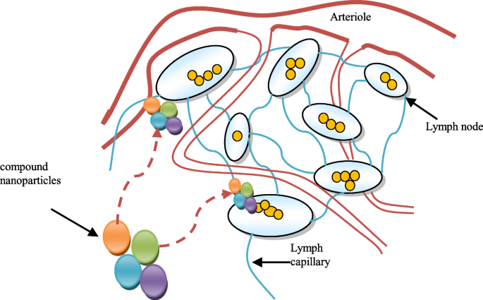
Sistema de administración de fármacos de nanopartículas compuestas y su interacción con los ganglios linfáticos

La Administración de Drogas y Alimentos de los Estados Unidos alude a los nanomateriales como materiales con partículas en el rango de 1 a 100 con propiedades diferentes del material a granel [4, 5]. Se han caracterizado nanofibras, nanoplacas, nanocables, puntos cuánticos y otros materiales relacionados [6]. Las nanopartículas de lípidos sólidos (SLN) son un tipo de nanopartículas de lípidos (NL), que pueden construirse utilizando lípidos sólidos [7]. Se han desarrollado versiones posteriores de SLN, como los portadores de lípidos nanoestructurados (NLC), que representan la segunda era de LN [8]. Tanto SLN como NLC se construyen a partir de lípidos sólidos. La estructura interior de SLN contiene lípidos sólidos, mientras que la NLC se desarrolla utilizando una mezcla de lípidos sólidos y líquidos, que producen una sección transversal de piedra preciosa [9, 10]. Estos defectos también se han informado para los GC a la luz del hecho de que los GC que contienen muchos segmentos de lípidos sólidos se pueden utilizar en aplicaciones médicas [11, 12]. Las nanopartículas poliméricas (PN) se pueden construir a partir de polímeros naturales o materiales inorgánicos, por ejemplo, sílice [13]. Los polímeros o lípidos dan forma al núcleo de las NP, que mejoran la estabilidad y la administración de fármacos y ofrecen una forma y tamaño uniformes [14]. La PN se puede describir como nanocápsulas o nanoesferas. Las nanocápsulas contienen aceite en una estructura vesicular junto con un fármaco [15, 16], mientras que las nanoesferas contienen cadenas poliméricas sin aceite [17, 18]. Un fármaco se envasa en NP mediante mezcla con el polímero. La incorporación del fármaco está asegurada en las nanopartículas en el momento de la polimerización. Los NP se cargan con un fármaco disolviéndolo, dispersándolo o adsorbiéndolo artificialmente en los constituyentes de la red polimérica [19, 20]. Hay tres tipos de linfocitos:células B, células T y células asesinas naturales. Las células B producen anticuerpos que atacan a los microorganismos invasores, mientras que también atacan el sistema inmunológico cuando se vuelven cancerígenos. Por lo tanto, considerando el importante papel del líquido linfático en la autoinmunidad, el objetivo de este trabajo fue diseñar un sistema inteligente de administración de fármacos basado en partículas de nanoantenas. Por tanto, el sistema contiene muchas nanopartículas en diferentes cantidades. La siguiente sección presenta el diseño de un sistema inteligente de administración de fármacos.

Diseño de un sistema de administración de fármacos nanointeligente

El sistema de administración de fármacos nanointeligente propuesto contiene un nanocontrolador operado por una fuente eléctrica de nanopartículas hechas de un material nano-piezoeléctrico. El complejo repositorio de nanopartículas tiene varios microdepósitos. Cada pequeño depósito contiene un tipo de nanopartículas. Una molécula de nanopartículas contiene una nanoantena diseñada para comunicarse con el nanocontrolador. El sistema de administración de fármacos nanointeligente propuesto también contiene nanotubos de carbono para la administración rápida de fármacos a las células cancerosas. Puede asociarse con las células infectadas como se muestra en la Fig. 2. El sistema comienza enviando nanopartículas a las células cancerosas llamadas "nanopartículas exploratorias". Estas moléculas, mediante comunicación anaeróbica, envían la imagen completa de su posición dentro de las células al nanocontrolador. Según la situación encontrada por las nanopartículas exploratorias, el nanocontrolador envía nanopartículas de diferente número, tipo y densidad a las células cancerosas, basándose en la información recopilada de las nanopartículas exploratorias. Estas nanopartículas se denominan "nanopartículas de combate".

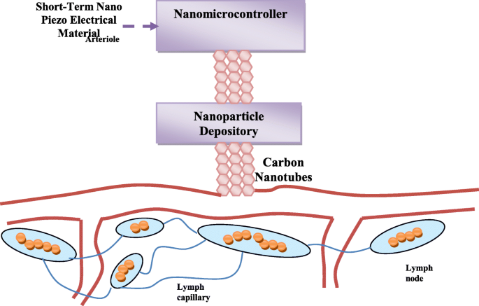
Estructura general que muestra la asociación del sistema farmacológico propuesto con las células infectadas

Este no es un proceso aleatorio, sino que está controlado por el nanocontrolador considerando varios aspectos y logaritmos, lo que garantizará una entrega eficiente y rápida de las nanopartículas. Para entregar con precisión y rapidez las nanopartículas a las células cancerosas, se empleará el algoritmo de búsqueda binaria compresiva [21]. Además, las nanopartículas se administrarán en diferentes densidades para que el fármaco sea más eficaz. Estas metodologías y su modus operandi al emplear el nanocontrolador se ilustran en la Fig. 3. La estructura física del nanocontrolador es similar a la de las nanopartículas, pero tiene forma de metal para que pueda ganar energía eléctrica. durante un breve período de tiempo mientras trabaja. Este metal contiene una antena inalámbrica junto con una pequeña memoria que contiene los códigos operativos con un enlace de nanopartículas entre el nanocontrolador y el almacén de nanopartículas. El depósito de nanopartículas contiene varios tipos diferentes de nanopartículas. La apertura y el cierre, así como la duración de la apertura de la nanopuerta, se controlarán para adaptar la cantidad de partículas que se entregarán.

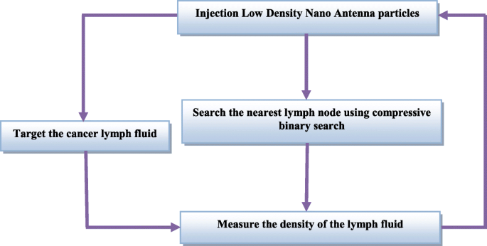
Proceso de envío de nanopartículas combatientes a las células cancerosas

Una descripción de la naturaleza de las nanopartículas utilizadas en el sistema de fármacos propuesto

En la siguiente sección, se discute la naturaleza de las nanopartículas utilizadas en el sistema de administración de fármacos propuesto. En este trabajo, se utilizaron nanopartículas anaeróbicas de baja densidad como se describe en un informe anterior [22].

Nanopartículas de baja densidad

Considere el proceso de administración de fármacos de nanopartículas compuestas para el cáncer como un proceso de penetración en el líquido linfático, donde un tumor está rodeado por el líquido linfático. La composición del melanoma se asemeja al líquido linfático. El modelo analítico propuesto se basa en un sistema de nanotubos que consta de tres tipos diferentes de nanopartículas. Las nanopartículas se colocan en un líquido linfático de alta densidad. Podemos definir nanopartículas específicas de sólido A en las coordenadas polares esféricas como A =(Ra, ϑ a , φa), donde ra es la coordenada radial de la nanopartícula del sólido A, ϑ a es la coordenada cenital de la nanopartícula del sólido A, y φa es la coordenada azimutal de la nanopartícula del sólido A. Las coordenadas correspondientes del sólido B son B =(Rb, ϑb, φb), respectivamente, y las coordenadas correspondientes de N sólido son N =(Rn, ϑn, φn), respectivamente. Tenga en cuenta que hay dos propiedades del ganglio linfático, es decir, sensible e hinchado, que se ven afectadas por las células cancerosas del linfoma de Hodgkin. El ganglio linfático con la propiedad sensible Tp se puede describir como Tp ( N , t ); esto significa que el valor de Tp en asociación con el fluido de nanopartículas de N sólido varía con el tiempo. Ahora, consideremos que el efecto total de las nanopartículas compuestas en la propiedad tierna se define como:

$$ \ mathrm {Tpt} =\ mathrm {Tp} \ \ left (A, t \ right) + \ mathrm {Tp} \ \ left (B, t \ right) +. \ puntos \ puntos \ puntos \ puntos + \ mathrm {Tp} \ \ left (N, t \ right) $$ (1)

Considere el mismo caso para la propiedad hinchada, que podría definirse como:

$$ \ mathrm {Tst} =\ mathrm {Ts} \ \ left (A, t \ right) + \ mathrm {Ts} \ \ left (B, t \ right) +. \ puntos \ puntos \ puntos \ puntos + \ mathrm {Ts} \ \ left (N, t \ right) $$ (2)

De las Ecs. 1 y 2, la tasa de cambio de ambas propiedades con el tiempo se puede determinar como:

$$ \ frac {\ parcial \ izquierda (\ mathrm {Tp} \ left (A, t \ derecha) \ derecha)} {\ parcial t} + \ frac {\ parcial \ izquierda (\ mathrm {Tp} \ left ( B, t \ derecha) \ derecha)} {\ t parcial} + \ puntos \ frac {\ parcial \ izquierda (\ mathrm {Tp} \ izquierda (N, t \ derecha) \ derecha)} {\ t parcial} =\ frac {\ mathrm {\ Tp parcial} (t)} {\ mathrm {\ t parcial}} $$ (3) $$ \ frac {\ parcial \ left (\ mathrm {Ts} \ left (A, t \ derecha) \ derecha)} {\ t parcial} + \ frac {\ parcial \ izquierda (\ mathrm {Ts} \ izquierda (B, t \ derecha) \ derecha)} {\ t parcial} + \ puntos \ frac {\ parcial \ izquierda (\ mathrm {Ts} \ izquierda (N, t \ derecha) \ derecha)} {\ parcial t} =\ frac {\ mathrm {\ parcial Ts} (t)} {\ parcial t} $$ ( 4)

El punto del líquido linfático que puede ocupar una nanopartícula de N sólido se define como:

$$ {\ mathrm {Po}} _ n =\ mathrm {Po} {\ izquierda (\ mathrm {po}, t \ derecha)} _ n $$ (5)

Consideremos que una nanopartícula del derivado sólido N del líquido linfático tierno se define como \ (\ frac {\ partial {\ left (\ mathrm {Tp} \ left (N, t \ right) \ right)} _ {\ mathrm {po}}} {\ parcial t} \), entonces el derivado del material compuesto del líquido linfático tierno sería igual a:

$$ \ frac {\ parcial {\ izquierda (\ mathrm {Tp} \ izquierda (A, t \ derecha) \ derecha)} _ {\ mathrm {po}}} {\ parcial t} + \ frac {\ parcial { \ izquierda (\ mathrm {Tp} \ izquierda (B, t \ derecha) \ derecha)} _ {\ mathrm {po}}} {\ t parcial} + \ puntos \ frac {\ parcial {\ izquierda (\ mathrm { Tp} \ izquierda (N, t \ derecha) \ derecha)} _ {\ mathrm {po}}} {\ t parcial} =\ frac {\ mathrm {\ tp parcial} {(t)} _ {\ mathrm { po}}} {\ t parcial} $$ (6) $$ \ frac {\ parcial {\ izquierda (\ mathrm {Ts} \ izquierda (A, t \ derecha) \ derecha)} _ {\ mathrm {po} }} {\ t parcial} + \ frac {\ parcial {\ izquierda (\ mathrm {Ts} \ izquierda (B, t \ derecha) \ derecha)} _ {\ mathrm {po}}} {\ t parcial} + \ puntos \ frac {\ parcial {\ izquierda (\ mathrm {Ts} \ izquierda (N, t \ derecha) \ derecha)} _ {\ mathrm {po}}} {\ parcial t} =\ frac {\ mathrm { \ T parcial} {(t)} _ {\ mathrm {po}}} {\ t parcial} $$ (7)

Los componentes de velocidad correspondientes del N sólido se toman como ( v _rn , v _ϑn , v _φn ). Luego, la velocidad de flujo de las partículas de N sólido se representa mediante las ecuaciones de Navier-Stokes a la viscosidad dinámica dν del líquido linfático y p es la presión y ρ es la densidad del líquido linfático de la siguiente manera:

$$ \ frac {\ parcial {v} _ {\ mathrm {rn}}} {\ parcial t} + {v} _ {\ mathrm {rn}} \ frac {\ parcial {v} _ {\ mathrm {rn }}} {\ mathrm {\ rn parcial}} + \ frac {v _ {\ upvartheta \ mathrm {n}}} {\ mathrm {rn}} \ frac {\ parcial {v} _ {\ mathrm {rn}} } {\ mathrm {\ parcial \ upvartheta n}} + \ frac {v _ {\ upvarphi \ mathrm {n}}} {\ mathrm {rn} \ \ mathrm {sin} \ upvartheta \ mathrm {n}} \ frac { \ parcial {v} _ {\ mathrm {rn}}} {\ mathrm {\ parcial \ upvarphi n}} - \ frac {v _ {\ upvartheta \ mathrm {n}} ^ 2} {\ mathrm {rn}} - \ frac {v _ {\ upvarphi \ mathrm {n}} ^ 2} {\ mathrm {rn}} + \ frac {1} {\ rho} \ frac {\ parcial p} {\ mathrm {\ parcial rn}} - \ mathrm {d} \ upnu \ left [\ frac {1} {{\ mathrm {rn}} ^ 2} \ frac {\ partial} {\ mathrm {\ partial rn}} \ left ({\ mathrm {rn} } ^ 2 \ frac {\ parcial {v} _ {\ mathrm {rn}}} {\ mathrm {\ parcial rn}} \ derecha) + \ frac {1} {{\ mathrm {rn}} ^ 2 \ mathrm {sin} \ upvartheta \ mathrm {n}} \ frac {\ partial} {\ mathrm {\ partial \ upvartheta n}} \ left (\ mathrm {sin} \ upvartheta \ mathrm {n} \ frac {\ partial {v } _ {\ mathrm {rn}}} {\ mathrm {\ parcial \ upvartheta n}} \ right) + \ frac {1} {{\ mathrm {rn}} ^ 2 {\ sin} ^ 2 \ upvartheta \ mathrm {n}} \ frac {\ parcial ^ 2 {v} _ {\ ma thrm {rn}}} {\ parcial {\ upvarphi \ mathrm {n}} ^ 2} + - \ frac {2 {v} _ {\ mathrm {rn}}} {{\ mathrm {rn}} ^ 2} - \ frac {2} {{\ mathrm {rn}} ^ 2 \ sin \ upvartheta \ mathrm {n}} \ frac {\ parcial \ left ({v} _ {\ upvartheta \ mathrm {n}} \ mathrm { sin} \ upvartheta \ mathrm {n} \ right)} {\ mathrm {\ partial \ upvartheta n}} - \ frac {2} {{\ mathrm {rn}} ^ 2 \ mathrm {sin} \ upvartheta \ mathrm { n}} \ frac {\ parcial {v} _ {\ upvarphi \ mathrm {n}}} {\ parcial _ {\ upvarphi \ mathrm {n}}} \ right] =0 $$ (8)

La viscosidad dinámica dν del líquido linfático se calcula de la siguiente manera:

Las ecuaciones de Navier-Stokes de los sólidos A y B podrían representarse como Ecs. 8 y 9. Por lo tanto, la ecuación. 9 podría representarse de la siguiente manera:

$$ \ mathrm {d} \ upnu =\ frac {\ izquierda [\ frac {\ parcial {v} _ {\ mathrm {rn}}} {\ parcial t} + {v} _ {\ mathrm {rn}} \ frac {\ parcial {v} _ {\ mathrm {rn}}} {\ mathrm {\ parcial rn}} + \ frac {v _ {\ upvartheta \ mathrm {n}}} {\ mathrm {rn}} \ frac {\ parcial {v} _ {\ mathrm {rn}}} {\ mathrm {\ parcial \ upvartheta n}} + \ frac {v _ {\ upvarphi \ mathrm {n}}} {\ mathrm {rn} \ \ mathrm {sin} \ upvartheta \ mathrm {n}} \ frac {\ parcial {v} _ {\ mathrm {rn}}} {\ mathrm {\ parcial \ upvarphi n}} - \ frac {v _ {\ upvartheta \ mathrm { n}} ^ 2} {\ mathrm {rn}} - \ frac {v _ {\ upvarphi \ mathrm {n}} ^ 2} {\ mathrm {rn}} + \ frac {1} {\ rho} \ frac { \ parcial p} {\ mathrm {\ parcial rn}} \ derecha]} {\ izquierda [\ frac {1} {{\ mathrm {rn}} ^ 2} \ frac {\ parcial} {\ mathrm {\ parcial rn }} \ izquierda ({\ mathrm {rn}} ^ 2 \ frac {\ parcial {v} _ {\ mathrm {rn}}} {\ mathrm {\ parcial rn}} \ derecha) + \ frac {1} { {\ mathrm {rn}} ^ 2 \ mathrm {sin} \ upvartheta \ mathrm {n}} \ frac {\ partial} {\ mathrm {\ partial \ upvartheta n}} \ left (\ mathrm {sin} \ upvartheta \ mathrm {n} \ frac {\ parcial {\ mathrm {v}} _ {\ mathrm {rn}}} {\ mathrm {\ partial \ upvartheta n}} \ right) + \ frac {1} {{\ mathrm { rn}} ^ 2 {\ sin} ^ 2 \ upvartheta \ math rm {n}} \ frac {\ parcial ^ 2 {\ mathrm {v}} _ {\ mathrm {rn}}} {\ parcial {\ upvarphi \ mathrm {n}} ^ 2} - \ frac {2 {\ mathrm {v}} _ {\ mathrm {rn}}} {{\ mathrm {rn}} ^ 2} - \ frac {2} {{\ mathrm {rn}} ^ 2 \ sin \ upvartheta \ mathrm {n} } \ frac {\ parcial \ izquierda ({\ mathrm {v}} _ {\ upvartheta \ mathrm {n}} \ mathrm {sin} \ upvartheta \ mathrm {n} \ right)} {\ mathrm {\ parcial \ upvartheta n}} - \ frac {2} {{\ mathrm {rn}} ^ 2 \ mathrm {sin} \ upvartheta \ mathrm {n}} \ frac {\ partial {\ mathrm {v}} _ {\ upvarphi \ mathrm {n}}} {\ parcial _ {\ upvarphi \ mathrm {n}}} \ derecha]} =\ frac {\ izquierda [\ frac {\ parcial {\ mathrm {v}} _ {\ mathrm {ra}}} {\ mathrm {\ parcial t}} + {\ mathrm {v}} _ {\ mathrm {ra}} \ frac {\ parcial {\ mathrm {v}} _ {\ mathrm {ra}}} {\ mathrm { \ parcial ra}} + \ frac {{\ mathrm {v}} _ {\ upvartheta \ mathrm {a}}} {\ mathrm {ra}} \ frac {\ parcial {\ mathrm {v}} _ {\ mathrm {ra}}} {\ mathrm {\ parcial \ upvartheta a}} + \ frac {{\ mathrm {v}} _ {\ upvarphi \ mathrm {a}}} {\ mathrm {ra} \ \ mathrm {sin} \ upvartheta \ mathrm {a}} \ frac {\ partial {\ mathrm {v}} _ {\ mathrm {ra}}} {\ mathrm {\ partial \ upvarphi a}} - \ frac {{\ mathrm {v} } _ {\ upvartheta \ mathrm {a}} ^ 2} {\ mathrm {ra}} - \ frac {{\ mathrm {v}} _ {\ upvarphi \ mathrm {a}} ^ 2} {\ mathrm {ra}} + \ frac {1} {\ uprho} \ frac {\ mathrm {\ parcial p} } {\ mathrm {\ parcial ra}} \ derecha]} {\ izquierda [\ frac {1} {{\ mathrm {ra}} ^ 2} \ frac {\ parcial} {\ mathrm {\ parcial ra}} \ izquierda ({\ mathrm {ra}} ^ 2 \ frac {\ parcial {v} _ {\ mathrm {ra}}} {\ mathrm {\ parcial ra}} \ derecha) + \ frac {1} {{\ mathrm {ra}} ^ 2 \ mathrm {sin} \ upvartheta \ mathrm {a}} \ frac {\ partial} {\ mathrm {\ partial \ upvartheta a}} \ left (\ mathrm {sin} \ upvartheta \ mathrm {a } \ frac {\ parcial {v} _ {\ mathrm {ra}}} {\ mathrm {\ parcial \ upvartheta a}} \ derecha) + \ frac {1} {{\ mathrm {ra}} ^ 2 {\ pecado} ^ 2 \ upvartheta \ mathrm {a}} \ frac {\ parcial ^ 2 {v} _ {\ mathrm {ra}}} {\ parcial {\ upvarphi \ mathrm {a}} ^ 2} - \ frac { 2 {v} _ {\ mathrm {ra}}} {{\ mathrm {ra}} ^ 2} - \ frac {2} {{\ mathrm {ra}} ^ 2 \ sin \ upvartheta \ mathrm {a}} \ frac {\ parcial \ izquierda ({v} _ {\ upvartheta \ mathrm {a}} \ mathrm {sin} \ upvartheta \ mathrm {a} \ right)} {\ mathrm {\ parcial \ upvartheta a}} - \ frac {2} {{\ mathrm {ra}} ^ 2 \ mathrm {sin} \ upvartheta \ mathrm {a}} \ frac {\ parcial {v} _ {\ upvarphi \ mathrm {a}}} {\ parcial_ { \ upvarphi \ mathrm {a}}} \ right]} =\ frac { \ izquierda [\ frac {\ parcial {v} _ {\ mathrm {rb}}} {\ parcial t} + {v} _ {\ mathrm {rb}} \ frac {\ parcial {v} _ {\ mathrm { rb}}} {\ mathrm {\ rb parcial}} + \ frac {v _ {\ upvartheta \ mathrm {b}}} {\ mathrm {rb}} \ frac {\ parcial {v} _ {\ mathrm {rb} }} {\ mathrm {\ parcial \ upvartheta b}} + \ frac {v _ {\ upvarphi \ mathrm {b}}} {\ mathrm {rb} \ \ mathrm {sin} \ upvartheta \ mathrm {b}} \ frac {\ parcial {v} _ {\ mathrm {rb}}} {\ mathrm {\ parcial \ upvarphi b}} - \ frac {v _ {\ upvartheta \ mathrm {b}} ^ 2} {\ mathrm {rb}} - \ frac {v _ {\ upvarphi \ mathrm {b}} ^ 2} {\ mathrm {rb}} + \ frac {1} {\ rho} \ frac {\ parcial p} {\ mathrm {\ parcial rb}} \ right]} {\ left [\ frac {1} {{\ mathrm {rb}} ^ 2} \ frac {\ partial} {\ mathrm {\ partial rb}} \ left ({\ mathrm {rb}} ^ 2 \ frac {\ parcial {v} _ {\ mathrm {rb}}} {\ mathrm {\ parcial rb}} \ derecha) + \ frac {1} {{\ mathrm {rb}} ^ 2 \ mathrm {sin } \ upvartheta \ mathrm {b}} \ frac {\ partial} {\ mathrm {\ partial \ upvartheta b}} \ left (\ mathrm {sin} \ upvartheta \ mathrm {b} \ frac {\ partial {v} _ {\ mathrm {rb}}} {\ mathrm {\ partial \ upvartheta b}} \ right) + \ frac {1} {{\ mathrm {rb}} ^ 2 {\ sin} ^ 2 \ upvartheta \ mathrm {b }} \ frac {\ parcial ^ 2 {v} _ {\ mathrm { rb}}} {\ parcial {\ upvarphi \ mathrm {b}} ^ 2} - \ frac {2 {v} _ {\ mathrm {rb}}} {{\ mathrm {rb}} ^ 2} - \ frac {2} {{\ mathrm {rb}} ^ 2 \ sin \ upvartheta \ mathrm {b}} \ frac {\ parcial \ left ({v} _ {\ upvartheta \ mathrm {b}} \ mathrm {sin} \ upvartheta \ mathrm {b} \ right)} {\ mathrm {\ parcial \ upvartheta b}} - \ frac {2} {{\ mathrm {rb}} ^ 2 \ mathrm {sin} \ upvartheta \ mathrm {b}} \ frac {\ parcial {v} _ {\ upvarphi \ mathrm {b}}} {\ parcial _ {\ upvarphi \ mathrm {b}}} \ right]} $$ (10)

Las partículas están en nano-dimensiones; por lo tanto, sus radios serían muy pequeños y, para simplificar, la ecuación. 10 se representa de la siguiente manera:

$$ \ mathrm {d} \ upnu =\ left [\ frac {v _ {\ upvartheta \ mathrm {n}}} {\ mathrm {rn}} \ frac {\ parcial {v} _ {\ mathrm {rn}} } {\ mathrm {\ parcial \ upvartheta n}} + \ frac {v _ {\ upvarphi \ mathrm {n}}} {\ mathrm {rn} \ \ mathrm {sin} \ upvartheta \ mathrm {n}} \ frac { \ parcial {v} _ {\ mathrm {rn}}} {\ mathrm {\ parcial \ upvarphi n}} - \ frac {v _ {\ upvartheta \ mathrm {n}} ^ 2} {\ mathrm {rn}} - \ frac {v _ {\ upvarphi \ mathrm {n}} ^ 2} {\ mathrm {rn}} + \ frac {1} {\ rho} \ frac {\ parcial p} {\ mathrm {\ parcial rn}} \ derecha] / \ izquierda [\ frac {1} {{\ mathrm {rn}} ^ 2} \ frac {\ parcial} {\ mathrm {\ parcial rn}} \ izquierda ({\ mathrm {rn}} ^ 2 \ frac {\ parcial {v} _ {\ mathrm {rn}}} {\ mathrm {\ parcial rn}} \ derecha) + \ frac {1} {{\ mathrm {rn}} ^ 2 \ mathrm {sin} \ upvartheta \ mathrm {n}} \ frac {\ partial} {\ mathrm {\ partial \ upvartheta n}} \ left (\ mathrm {sin} \ upvartheta \ mathrm {n} \ frac {\ partial {\ mathrm {v} } _ {\ mathrm {rn}}} {\ mathrm {\ parcial \ upvartheta n}} \ right) + \ frac {1} {{\ mathrm {rn}} ^ 2 {\ sin} ^ 2 \ upvartheta \ mathrm {n}} \ frac {\ parcial ^ 2 {\ mathrm {v}} _ {\ mathrm {rn}}} {\ parcial {\ upvarphi \ mathrm {n}} ^ 2} - \ frac {2 {\ mathrm {v}} _ {\ mathrm {rn}}} {{\ math rm {rn}} ^ 2} - \ frac {2} {{\ mathrm {rn}} ^ 2 \ sin \ upvartheta \ mathrm {n}} \ frac {\ parcial \ izquierda ({\ mathrm {v}} _ {\ upvartheta \ mathrm {n}} \ mathrm {sin} \ upvartheta \ mathrm {n} \ right)} {\ mathrm {\ partial \ upvartheta n}} - \ frac {2} {{\ mathrm {rn}} ^ 2 \ mathrm {sin} \ upvartheta \ mathrm {n}} \ frac {\ partial {\ mathrm {v}} _ {\ upvarphi \ mathrm {n}}} {\ partial _ {\ upvarphi \ mathrm {n}} } \ derecha] =\ izquierda [\ frac {{\ mathrm {v}} _ {\ upvartheta \ mathrm {a}}} {\ mathrm {ra}} \ frac {\ parcial {\ mathrm {v}} _ { \ mathrm {ra}}} {\ mathrm {\ parcial \ upvartheta a}} + \ frac {{\ mathrm {v}} _ {\ upvarphi \ mathrm {a}}} {\ mathrm {ra} \ \ mathrm { sin} \ upvartheta \ mathrm {a}} \ frac {\ parcial {\ mathrm {v}} _ {\ mathrm {ra}}} {\ mathrm {\ parcial \ upvarphi a}} - \ frac {{\ mathrm { v}} _ {\ upvartheta \ mathrm {a}} ^ 2} {\ mathrm {ra}} - \ frac {{\ mathrm {v}} _ {\ upvarphi \ mathrm {a}} ^ 2} {\ mathrm {ra}} + \ frac {1} {\ uprho} \ frac {\ mathrm {\ parcial p}} {\ mathrm {\ parcial ra}} \ derecha] / \ izquierda [\ frac {1} {{\ mathrm {ra}} ^ 2} \ frac {\ parcial} {\ mathrm {\ parcial ra}} \ left ({\ mathrm {ra}} ^ 2 \ frac {\ parcial {\ mathrm {v}} _ {\ mathrm {ra}}} {\ mathrm {\ parcial ra}} \ rig ht) + \ frac {1} {{\ mathrm {ra}} ^ 2 \ mathrm {sin} \ upvartheta \ mathrm {a}} \ frac {\ partial} {\ mathrm {\ partial \ upvartheta a}} \ left (\ mathrm {sin} \ upvartheta \ mathrm {a} \ frac {\ parcial {\ mathrm {v}} _ {\ mathrm {ra}}} {\ mathrm {\ parcial \ upvartheta a}} \ derecha) + \ frac {1} {{\ mathrm {ra}} ^ 2 {\ sin} ^ 2 \ upvartheta \ mathrm {a}} \ frac {\ parcial ^ 2 {\ mathrm {v}} _ {\ mathrm {ra}} } {\ partial {\ upvarphi \ mathrm {a}} ^ 2} - \ frac {2 {\ mathrm {v}} _ {\ mathrm {ra}}} {{\ mathrm {ra}} ^ 2} - \ frac {2} {{\ mathrm {ra}} ^ 2 \ sin \ upvartheta \ mathrm {a}} \ frac {\ parcial \ left ({\ mathrm {v}} _ {\ upvartheta \ mathrm {a}} \ mathrm {sin} \ upvartheta \ mathrm {a} \ right)} {\ mathrm {\ partial \ upvartheta a}} - \ frac {2} {{\ mathrm {ra}} ^ 2 \ mathrm {sin} \ upvartheta \ mathrm {a}} \ frac {\ parcial {v} _ {\ upvarphi \ mathrm {a}}} {\ partial _ {\ upvarphi \ mathrm {a}}} \ right] =\ left [\ frac {v _ {\ upvartheta \ mathrm {b}}} {\ mathrm {rb}} \ frac {\ parcial {v} _ {\ mathrm {rb}}} {\ mathrm {\ parcial \ upvartheta b}} + \ frac {v _ {\ upvarphi \ mathrm {b}}} {\ mathrm {rb} \ \ mathrm {sin} \ upvartheta \ mathrm {b}} \ frac {\ parcial {v} _ {\ mathrm {rb}}} {\ mathrm {\ parcial \ upvarphi b}} - \ frac {v _ {\ upvartheta \ mathrm {b}} ^ 2} {\ mathrm {rb}} - \ frac {v _ {\ upvarphi \ mathrm {b}} ^ 2} {\ mathrm {rb }} + \ frac {1} {\ rho} \ frac {\ parcial p} {\ mathrm {\ parcial rb}} \ derecha] / \ izquierda [\ frac {1} {{\ mathrm {rb}} ^ 2 } \ frac {\ parcial} {\ mathrm {\ parcial rb}} \ izquierda ({\ mathrm {rb}} ^ 2 \ frac {\ parcial {v} _ {\ mathrm {rb}}} {\ mathrm {\ parcial rb}} \ derecha) + \ frac {1} {{\ mathrm {rb}} ^ 2 \ mathrm {sin} \ upvartheta \ mathrm {b}} \ frac {\ parcial} {\ mathrm {\ parcial \ upvartheta b}} \ izquierda (\ mathrm {sin} \ upvartheta \ mathrm {b} \ frac {\ parcial {v} _ {\ mathrm {rb}}} {\ mathrm {\ parcial \ upvartheta b}} \ derecha) + \ frac {1} {{\ mathrm {rb}} ^ 2 {\ sin} ^ 2 \ upvartheta \ mathrm {b}} \ frac {\ partial ^ 2 {v} _ {\ mathrm {rb}}} {\ parcial {\ upvarphi \ mathrm {b}} ^ 2} - \ frac {2 {v} _ {\ mathrm {rb}}} {{\ mathrm {rb}} ^ 2} - \ frac {2} {{\ mathrm {rb}} ^ 2 \ sin \ upvartheta \ mathrm {b}} \ frac {\ parcial \ left ({v} _ {\ upvartheta \ mathrm {b}} \ mathrm {sin} \ upvartheta \ mathrm {b} \ right)} {\ mathrm {\ partial \ upvartheta b}} - \ frac {2} {{\ mathrm {rb}} ^ 2 \ mathrm {sin} \ upvartheta \ mathrm {b}} \ frac {\ partial { v} _ {\ upvarphi \ mathrm {b}}} {\ parcial _ {\ upvarphi \ mathrm {b}}} \ right] $$ (11)

La ecuación 11 podría representarse de la siguiente manera:

$$ \ mathrm {d} \ upnu =\ mathrm {rn} \ left [{v} _ {\ upvartheta \ mathrm {n}} \ frac {\ partial {v} _ {\ mathrm {rn}}} {\ mathrm {\ parcial \ upvartheta n}} + \ frac {v _ {\ upvarphi \ mathrm {n}}} {\ \ mathrm {sin} \ upvartheta \ mathrm {n}} \ frac {\ parcial {v} _ {\ mathrm {rn}}} {\ mathrm {\ parcial \ upvarphi n}} - {v} _ {\ upvartheta \ mathrm {n}} ^ 2- {v} _ {\ upvarphi \ mathrm {n}} ^ 2+ \ frac {\ mathrm {rn}} {\ rho} \ frac {\ parcial p} {\ mathrm {\ parcial rn}} \ derecha] / \ izquierda [\ frac {\ parcial} {\ mathrm {\ parcial rn} } \ izquierda ({\ mathrm {rn}} ^ 2 \ frac {\ parcial {v} _ {\ mathrm {rn}}} {\ mathrm {\ parcial rn}} \ derecha) + \ frac {1} {\ mathrm {sin} \ upvartheta \ mathrm {n}} \ frac {\ partial} {\ mathrm {\ partial \ upvartheta n}} \ left (\ mathrm {sin} \ upvartheta \ mathrm {n} \ frac {\ partial { v} _ {\ mathrm {rn}}} {\ mathrm {\ parcial \ upvartheta n}} \ right) + \ frac {1} {\ sin ^ 2 \ upvartheta \ mathrm {n}} \ frac {\ parcial ^ 2 {v} _ {\ mathrm {rn}}} {\ parcial {\ upvarphi \ mathrm {n}} ^ 2} -2 {v} _ {\ mathrm {rn}} - \ frac {2} {\ sin \ upvartheta \ mathrm {n}} \ frac {\ partial \ left ({v} _ {\ upvartheta \ mathrm {n}} \ mathrm {sin} \ upvartheta \ mathrm {n} \ right)} {\ mathrm {\ par tial \ upvartheta n}} - \ frac {2} {\ mathrm {sin} \ upvartheta \ mathrm {n}} \ frac {\ parcial {v} _ {\ upvarphi \ mathrm {n}}} {\ parcial _ {\ upvarphi \ mathrm {n}}} \ right] =\ mathrm {ra} \ left [{v} _ {\ upvartheta \ mathrm {a}} \ frac {\ parcial {v} _ {\ mathrm {ra}}} {\ mathrm {\ parcial \ upvartheta a}} + \ frac {v _ {\ upvarphi \ mathrm {a}}} {\ \ mathrm {sin} \ upvartheta \ mathrm {a}} \ frac {\ parcial {v} _ {\ mathrm {ra}}} {\ mathrm {\ parcial \ upvarphi a}} - {v} _ {\ upvartheta \ mathrm {a}} ^ 2- {v} _ {\ upvarphi \ mathrm {a}} ^ 2+ \ frac {\ mathrm {ra}} {\ rho} \ frac {\ parcial p} {\ mathrm {\ parcial ra}} \ derecha] / \ izquierda [\ frac {\ parcial} {\ mathrm {\ parcial ra}} \ izquierda ({\ mathrm {ra}} ^ 2 \ frac {\ parcial {v} _ {\ mathrm {ra}}} {\ mathrm {\ parcial ra}} \ derecha) + \ frac {1} {\ mathrm {sin} \ upvartheta \ mathrm {a}} \ frac {\ parcial} {\ mathrm {\ parcial \ upvartheta a}} \ left (\ mathrm {sin} \ upvartheta \ mathrm {a} \ frac {\ parcial {v} _ {\ mathrm {ra}}} {\ mathrm {\ parcial \ upvartheta a}} \ right) + \ frac {1} {\ sin ^ 2 \ upvartheta \ mathrm {a}} \ frac {\ parcial ^ 2 {v} _ {\ mathrm {ra}}} {\ parcial {\ upvarphi \ mathrm {a}} ^ 2} -2 {v} _ {\ mathrm {ra}} - \ frac {2} { \pecado \ upvartheta \ mathrm {a}} \ frac {\ partial \ left ({v} _ {\ upvartheta \ mathrm {a}} \ mathrm {sin} \ upvartheta \ mathrm {a} \ right)} {\ mathrm {\ parcial \ upvartheta a}} - \ frac {2} {\ mathrm {sin} \ upvartheta \ mathrm {a}} \ frac {\ parcial {v} _ {\ upvarphi \ mathrm {a}}} {\ parcial _ {\ upvarphi \ mathrm {a}}} \ right] =\ mathrm {rb} \ left [{v} _ {\ upvartheta \ mathrm {b}} \ frac {\ parcial {v} _ {\ mathrm {rb}}} {\ mathrm {\ parcial \ upvartheta b}} + \ frac {v _ {\ upvarphi \ mathrm {b}}} {\ \ mathrm {sin} \ upvartheta \ mathrm {b}} \ frac {\ parcial {v} _ {\ mathrm {rb}}} {\ mathrm {\ parcial \ upvarphi b}} - {v} _ {\ upvartheta \ mathrm {b}} ^ 2- {v} _ {\ upvarphi \ mathrm {b}} ^ 2+ \ frac {\ mathrm {rb}} {\ rho} \ frac {\ parcial p} {\ mathrm {\ parcial rb}} \ derecha] / \ izquierda [\ frac {\ parcial} {\ mathrm {\ parcial rb}} \ izquierda ({\ mathrm {rb}} ^ 2 \ frac {\ parcial {v} _ {\ mathrm {rb}}} {\ mathrm {\ parcial rb}} \ derecha) + \ frac {1} {\ mathrm {sin} \ upvartheta \ mathrm {b}} \ frac {\ parcial} {\ mathrm {\ parcial \ upvartheta b}} \ left (\ mathrm {sin} \ upvartheta \ mathrm {b} \ frac {\ parcial {v} _ {\ mathrm {rb}}} {\ mathrm {\ parcial \ upvartheta b}} \ derecha) + \ frac {1} {\ si n ^ 2 \ upvartheta \ mathrm {b}} \ frac {\ parcial ^ 2 {v} _ {\ mathrm {rb}}} {\ parcial {\ upvarphi \ mathrm {b}} ^ 2} -2 {v} _ {\ mathrm {rb}} - \ frac {2} {\ sin \ upvartheta \ mathrm {b}} \ frac {\ parcial \ left ({v} _ {\ upvartheta \ mathrm {b}} \ mathrm {sin } \ upvartheta \ mathrm {b} \ right)} {\ mathrm {\ partial \ upvartheta b}} - \ frac {2} {\ mathrm {sin} \ upvartheta \ mathrm {b}} \ frac {\ partial {v } _ {\ upvarphi \ mathrm {b}}} {\ parcial _ {\ upvarphi \ mathrm {b}}} \ right] $$ (12)

Existe una relación directa entre los radios de las nanopartículas y la viscosidad linfática debida al cáncer. Si la linfa se vuelve demasiado estática y viscosa, no puede llevar a cabo su función correctamente, que es la de circular y limpiar las toxinas y ayudar a combatir el cáncer. Si el tamaño de las nanopartículas es más pequeño, las células cancerosas linfáticas son fáciles de matar. Para describir el transporte de la cantidad total de nanopartículas compuestas, usamos la ecuación de continuidad y asumimos las tres nanopartículas de sólidos A, B y N de la siguiente manera:

$$ \ frac {1} {{\ mathrm {ra}} ^ 2} \ frac {\ parcial} {\ mathrm {\ parcial ra}} \ left ({\ mathrm {ra}} ^ 2 {v} _ { \ mathrm {ra}} \ derecha) + \ frac {1} {\ mathrm {ra} \ \ mathrm {sin} \ upvartheta \ mathrm {a}} \ frac {\ parcial} {\ mathrm {\ parcial \ upvartheta a }} \ left (\ sin {\ upvartheta \ mathrm {v}} _ {\ upvartheta \ mathrm {a}} \ right) + \ frac {1} {\ mathrm {ra} \ \ mathrm {sin} \ upvartheta \ mathrm {a}} \ frac {\ parcial {v} _ {\ upvarphi \ mathrm {a}}} {\ mathrm {\ parcial \ upvarphi a}} + \ frac {1} {{\ mathrm {rb}} ^ 2} \ frac {\ parcial} {\ mathrm {\ parcial rb}} \ left ({\ mathrm {rb}} ^ 2 {v} _ {\ mathrm {rb}} \ right) + \ frac {1} { \ mathrm {rb} \ \ mathrm {sin} \ upvartheta \ mathrm {b}} \ frac {\ partial} {\ mathrm {\ partial \ upvartheta b}} \ left (\ sin {\ upvartheta v} _ {\ upvartheta \ mathrm {b}} \ right) + \ frac {1} {\ mathrm {rb} \ \ mathrm {sin} \ upvartheta \ mathrm {b}} \ frac {\ parcial {v} _ {\ upvarphi \ mathrm { b}}} {\ mathrm {\ parcial \ upvarphi b}} + \ frac {1} {{\ mathrm {rn}} ^ 2} \ frac {\ parcial} {\ mathrm {\ parcial rn}} \ left ( {\ mathrm {rn}} ^ 2 {v} _ {\ mathrm {rn}} \ right) + \ frac {1} {\ mathrm {rn} \ \ mathrm {sin} \ upvartheta \ mathrm {n}} \ frac {\ parti al} {\ mathrm {\ parcial \ upvartheta n}} \ left (\ sin {\ upvartheta v} _ {\ upvartheta \ mathrm {n}} \ right) + \ frac {1} {\ mathrm {rn} \ \ mathrm {sin} \ upvartheta \ mathrm {n}} \ frac {\ partial {v} _ {\ upvarphi \ mathrm {n}}} {\ mathrm {\ partial \ upvarphi n}} =0 $$ (13)

La viscosidad dinámica del fluido se puede determinar a partir de la siguiente ecuación [23]:

$$ \ mathrm {Vs} =\ frac {2} {9} \ frac {r ^ 2g \ \ left (\ uprho \ mathrm {p} - \ uprho \ mathrm {f} \ right)} {\ mathrm {dv }} $$ (14)

where Vs is the particles’ settling velocity (m/s), r is the Stokes radius of the particle (m), g is the gravitational acceleration (m/s² ), ρp is the density of the particles (kg/m³ ), ρf is the density of the fluid (kg/m³ ), and dv is the (dynamic) fluid viscosity (Pa·s). The lymph fluid is slightly heavier than water (lymph density = 1019 kg/m³ , water density = 998.28 kg/m³ at 20 °C). As a reference value, we consider the dynamic viscosity of the water to be 1.002 × 10^–3 kg m^–1 s^–1 ).

Dynamic viscosity is the measurement of the fluid’s internal resistance to flow, while kinematic viscosity refers to the ratio of dynamic viscosity to density. The effect of all the nanoparticles on the fluid viscosity is represented as follows:

$$ \mathrm{dv}=\frac{2\mathrm{g}}{9}\left[\frac{{\mathrm{ra}}^2\left(\uprho \mathrm{a}-\uprho \mathrm{f}\right)}{\mathrm{vsa}}+\frac{{\mathrm{rb}}^2\left(\uprho \mathrm{b}-\uprho \mathrm{f}\right)}{\mathrm{vsb}}+\frac{{\mathrm{rn}}^2\left(\uprho \mathrm{n}-\uprho \mathrm{f}\right)}{\mathrm{vn}}\right] $$ (15)

By comparing Eq. 12 and Eq. 15, the following equation could be emerged:

$$ \left|\frac{2\mathrm{g}}{9}\left[\frac{{\mathrm{ra}}^2\left(\uprho \mathrm{a}-\uprho \mathrm{f}\right)}{\mathrm{vsa}}+\frac{{\mathrm{rb}}^2\left(\uprho \mathrm{b}-\uprho \mathrm{f}\right)}{\mathrm{vsb}}+\frac{{\mathrm{rn}}^2\left(\uprho \mathrm{n}-\uprho \mathrm{f}\right)}{\mathrm{vn}}\right]\right|=\mathrm{rn}\left[{v}_{\upvartheta \mathrm{n}}\frac{\partial {v}_{\mathrm{rn}}}{\mathrm{\partial \upvartheta n}}+\frac{v_{\upvarphi \mathrm{n}}}{\ \mathrm{sin}\upvartheta \mathrm{n}}\frac{\partial {v}_{\mathrm{rn}}}{\mathrm{\partial \upvarphi n}}-{v}_{\upvartheta \mathrm{n}}^2-{v}_{\upvarphi \mathrm{n}}^2+\frac{\mathrm{rn}}{\uprho \mathrm{f}}\frac{\mathrm{\partial p}}{\mathrm{\partial rn}}\right]/\left[\frac{\partial }{\mathrm{\partial rn}}\left({\mathrm{rn}}^2\frac{\partial {v}_{\mathrm{rn}}}{\mathrm{\partial rn}}\right)+\frac{1}{\mathrm{sin}\upvartheta \mathrm{n}}\frac{\partial }{\mathrm{\partial \upvartheta n}}\left(\mathrm{sin}\upvartheta \mathrm{n}\frac{\partial {v}_{\mathrm{rn}}}{\mathrm{\partial \upvartheta n}}\right)+\frac{1}{\sin^2\upvartheta \mathrm{n}}\frac{\partial^2{v}_{\mathrm{rn}}}{\partial {\upvarphi \mathrm{n}}^2}-2{v}_{\mathrm{rn}}-\frac{2}{\sin \upvartheta \mathrm{n}}\frac{\partial \left({v}_{\upvartheta \mathrm{n}}\mathrm{sin}\upvartheta \mathrm{n}\right)}{\mathrm{\partial \upvartheta n}}-\frac{2}{\mathrm{sin}\upvartheta \mathrm{n}}\frac{\partial {v}_{\upvarphi \mathrm{n}}}{\partial_{\upvarphi \mathrm{n}}}\right]=\mathrm{ra}\left[{v}_{\upvartheta \mathrm{a}}\frac{\partial {v}_{\mathrm{ra}}}{\mathrm{\partial \upvartheta a}}+\frac{v_{\upvarphi \mathrm{a}}}{\ \mathrm{sin}\upvartheta \mathrm{a}}\frac{\partial {v}_{\mathrm{ra}}}{\mathrm{\partial \upvarphi a}}-{v}_{\upvartheta \mathrm{a}}^2-{v}_{\upvarphi \mathrm{a}}^2+\frac{\mathrm{ra}}{\uprho \mathrm{f}}\frac{\partial p}{\mathrm{\partial ra}}\right]/\left[\frac{\partial }{\mathrm{\partial ra}}\left({\mathrm{ra}}^2\frac{\partial {v}_{\mathrm{ra}}}{\mathrm{\partial ra}}\right)+\frac{1}{\mathrm{sin}\upvartheta \mathrm{a}}\frac{\partial }{\mathrm{\partial \upvartheta a}}\left(\mathrm{sin}\upvartheta \mathrm{a}\frac{\partial {v}_{\mathrm{ra}}}{\mathrm{\partial \upvartheta a}}\right)+\frac{1}{\sin^2\upvartheta \mathrm{a}}\frac{\partial^2{v}_{\mathrm{ra}}}{\partial {\upvarphi \mathrm{a}}^2}-2{v}_{\mathrm{ra}}-\frac{2}{\sin \upvartheta \mathrm{a}}\frac{\partial \left({v}_{\upvartheta \mathrm{a}}\mathrm{sin}\upvartheta \mathrm{a}\right)}{\mathrm{\partial \upvartheta a}}-\frac{2}{\mathrm{sin}\upvartheta \mathrm{a}}\frac{\partial {v}_{\upvarphi \mathrm{a}}}{\partial_{\upvarphi \mathrm{a}}}\right]=\mathrm{rb}\left[{v}_{\upvartheta \mathrm{b}}\frac{\partial {v}_{\mathrm{rb}}}{\mathrm{\partial \upvartheta b}}+\frac{v_{\upvarphi \mathrm{b}}}{\ \mathrm{sin}\upvartheta \mathrm{b}}\frac{\partial {v}_{\mathrm{rb}}}{\mathrm{\partial \upvarphi b}}-{v}_{\upvartheta \mathrm{b}}^2-{v}_{\upvarphi \mathrm{b}}^2+\frac{\mathrm{rb}}{\uprho \mathrm{f}}\frac{\partial p}{\mathrm{\partial rb}}\right]/\left[\frac{\partial }{\mathrm{\partial rb}}\left({\mathrm{rb}}^2\frac{\partial {v}_{\mathrm{rb}}}{\mathrm{\partial rb}}\right)+\frac{1}{\mathrm{sin}\upvartheta \mathrm{b}}\frac{\partial }{\mathrm{\partial \upvartheta b}}\left(\mathrm{sin}\upvartheta \mathrm{b}\frac{\partial {v}_{\mathrm{rb}}}{\mathrm{\partial \upvartheta b}}\right)+\frac{1}{\sin^2\upvartheta \mathrm{b}}\frac{\partial^2{v}_{\mathrm{rb}}}{\partial {\upvarphi \mathrm{b}}^2}-2{v}_{\mathrm{rb}}-\frac{2}{\sin \upvartheta \mathrm{b}}\frac{\partial \left({v}_{\upvartheta \mathrm{b}}\mathrm{sin}\upvartheta \mathrm{b}\right)}{\mathrm{\partial \upvartheta b}}-\frac{2}{\mathrm{sin}\upvartheta \mathrm{b}}\frac{\partial {v}_{\upvarphi \mathrm{b}}}{\partial_{\upvarphi \mathrm{b}}}\right] $$ (16)

Equation 16 depicts the relationship between the density of the lymph fluid, the density of the nanoparticles of the compound drug system, and the radius of the nanoparticles. There is a positive correlation between the density of the lymph fluid and the density of the nanoparticles. The smaller the density and radius of nanoparticles, the lesser the density of the fluid will be. As established earlier, the decrease in the density of the lymph fluid leads to its inability to reproduce and reduce the ferocity of the disease. It can, therefore, be concluded that the tumor can be cured by minimizing the size of nanoparticles. These particles can reach in the range of up to 0.1 nm (i.e., Angstrom or picometer range). The particles of this size can act as the nucleus of drug delivery in this drug system. Equation 16 shows that radii of the nanoparticles in the proposed drug system are related to the effectiveness of the delivery system. Much lower sized nanoparticles can reduce the density of lymph fluid and the spread of the disease.

Nanoparticles with Nanoantennas

This study used the nanoparticle described in an earlier report [22] as an emissary with a nano-microcontroller. In the system, the proposed transmission distance is very small and compatible with the composition of nanoparticles. Thus, the middle gap can be neglected in mid-distance and is symbolized by C _d . Further, R _a and X _a are the real part and the imaginary part of the anaerobic impedance. After neglecting the load of the intercellular space between the nanoparticles and the nano-microcontroller, R _a and X _a can be calculated as follows [22]:

$$ {R}_a=\frac{r_{a0}}{1+{C}_d{w}_a\left(2{x}_{a0}+{C}_d\left({r_{a0}}^2+{x_{a0}}^2\right){w}_a\right)} $$ (17) $$ {X}_a=\frac{x_0-{C}_d\left({r_{a0}}^2+{x_{a0}}^2\right){w}_a}{1+{C}_d{w}_a\left(2{x}_{a0}+{C}_d\left({r_{a0}}^2+{x_{a0}}^2\right){w}_a\right)} $$ (18)

Thus, the load resistance value of nanotubes can be predicted as in the following equation:

$$ {r}_l=\frac{g^2R}{g^2-2 gSX{\varepsilon}_L\omega +{S}^2\left({R}^2+{X}^2\right){\varepsilon_L}^2{\omega}^2} $$ (19)

donde ε _L is the permittivity of the loading material, g is the size of the gap, and S is the effective cross-section area of the gap. In order to simplify the equation, the value of g ² can be neglected as it is too low and the final equation can be rewritten as follows:

$$ {r}_l=\frac{g^2R}{-2 gSX{\varepsilon}_L\omega +{S}^2\left({R}^2+{X}^2\right){\varepsilon_L}^2{\omega}^2} $$ (20)

Then,

$$ {r}_l=\frac{g^2R}{S{\varepsilon}_L\omega \left(-2 gX+S\left({R}^2+{X}^2\right){\varepsilon}_L\omega \right)} $$ (21)

The optical nano-photo concept can be used as an effective tool for interpreting and predicting these effects to design and improve nanoscale parameters and increase the nano-sensitivity to serve better as a single molecular sensor. Nanoantenna may provide optimal performance in terms of sensitivity, efficiency, and bandwidth in the process. The next section presents the concept of searching the cancerous lymph nodes using compressive binary search algorithm.

Searching for the Target Lymphatic Nodes Using Compressive Binary Search

In order for nanoparticles to reach the cancerous cells in a fast and efficient manner, we applied compressive binary search by the nano-microcontroller. The guided nanoparticles follow a specific path to quickly reach the target. This movement is based on the information obtained from the “exploratory nanoparticles.” Assume that the target lymph node, Tf, has exactly one nonzero entry, where the location of the lymph node is unknown. The algorithm divides mt measurements into a total of St stages, where St refers to the stages of the lymph nodes. The measurements are more than one for all the stages of the lymph nodes, which is necessary for the algorithm to be executed until completion. Based on this measurement, the algorithm decides between going left or right, until the nanoparticles reach the target, the cancerous lymph node.

Resultados y discusión

In order to analyze the proposed design, the nanoparticles were applied to the following five types of materials:silicone, lithium, lung, helium, and hydrogen. The materials were chosen because of their low density. The lung nanoparticles were samples from nano-sized lung nodules. They appear encircling with white shadows in a chest X-ray or computerized tomography scan taken from the lung of the person and required to be undamaged. The proposed idea is based on the analytical model, which indicates that the smaller the density of nanoparticles, the smaller the dynamic viscosity will be. This will result in a decrease in fluid viscosity. It is shown that the types of materials and the density of each particle will affect settling velocity of nanoparticles at entry into the lymphatic fluid and the density of the lymphatic fluid. We considered the following parameters:acceleration of gravity (g ) = 9.80665, particle diameter (d ) = 10 A, initial density of lymph fluid (ρf) = 998.28, and dynamic viscosity = 0.0010 kg m^–1 s^–1 [24]. These parameters were selected by the assumption that the viscosity of the lymphatic fluid is very similar to the viscosity of the water and the very small difference does not affect the results of the model. Figure 4 illustrates the density of nanoparticles for five selected materials for application in the proposed analytical model. Figure 5 shows the settling velocity for each particle. Figure 6 shows the effect of the settling velocity of nanoparticles on altering the lymphocyte density of cancer cells. The results shown in Fig. 6 show that the settling velocity of the particles carries a negative value. This indicates that the nanoparticle after entering in the lymphatic fluid rapidly moves in the opposite direction toward their entry into the lymphatic fluid. In general, any object that moves in the negative direction has a negative velocity. This movement of the particle leads to reduced viscosity of the lymphatic fluid.

Density of nanoparticles for the five selected materials

The settling velocity data for each particle

The effect of the settling velocity of nanoparticles on changing the lymphocyte density of cancer cells

Silicone nanoparticles showed the settling velocity of approximately − 2.87 × 10–15 m/s. This resulted in a decrease in viscosity of the lymphatic fluid to 987.72 kg/m³ for the initial density 998.28 kg/m³ . The density is continuously reduced to a point where hydrogen produces extremely spectacular results, i.e., the complete collapse of lymphatic fluid resistance. The density of the lymphatic fluid − 856.28 kg/m³ with the negative sign indicated that there was no resistance from the lymphatic fluid to the flow of the nanoparticles, resulting in the complete collapse of the liquid fluid. Both the hydrogen and helium particles have a significant impact on the liquid viscosity due to the low density of the particles. Hence, it is important to use a drug system consisting of a group of nanoparticles for low-density materials. Figure 7 shows the relationship between the diameters of lung nanoparticles and the number of nanoparticles in one group. The figure shows that the higher the diameter of nanoparticles, the fewer their number in a group. This is clearly shown at the highest value of the nanoparticle diameter of 1000 nm, where the number of molecules in a group is 20 molecules. Figure 8 shows the relationship between the diameters of lithium nanoparticles and the number of nanoparticles in one group. This figure demonstrates the inverse relationship between the radius of nanoparticles and the number of molecules in a group where lithium particle diameters are significantly lower than the lung nanoparticles, where the number of nanoparticles in Fig. 7 is relatively low compared to the lithium particles as shown in Fig. 8. And the multicolor balls in both figures refer to different ranges of nanoparticle radii for each group, where each group contains a number of nanoparticles with different sizes. The best results can be obtained when hydrogen and helium particles are increased from other substances. A mixture of different materials should be used so that the properties of these substances can be used in the treatment process as well as to reduce viscosity. Figure 9 illustrates the different sets of materials proposed to have the mean highest density of both hydrogen and helium materials. Figure 10 shows the average mass of a nanoparticle in a group. It can be seen that the mass of both hydrogen and helium is the highest compared to the mass of particles of other substances. Figure 11 illustrates the relationship between the diameters of the nanoparticles and the width of its group or class. It is important to note that these results will open up a new area to reduce the resistance of the lymphatic fluid in tumors. This can be achieved using hydrogen nanoparticles of a size in the range of Angstrom. In addition to hydrogen nanoparticles, there may also exist a number of other substances in the same size. Figure 12 illustrates the standard deviation of a number of coefficients for both lung and lithium nanoparticles. These coefficients are limited to fractions of nanoparticles in a single group as well as their number in addition to the diameters of these nanoparticles. It is clear that the group fractions have the less value of the standard deviation. Hence, most of the fractions in the computational processes are around the mean of these values. Figure 13 shows the standard deviation of the mass for particles of silicones, lithium, lungs, helium, and hydrogen in one group. It is clear that the particles of the lung have the largest standard deviation and the lithium has the minimum value.

Group of nanoparticles in the lung cells and their number in one of the proposed groups

Group of nanoparticles in the lithium cells and their number in one of the proposed groups

Different sets of materials proposed to have the mean highest density of both hydrogen and helium materials

Average mass of a nanoparticle in a group

Diameters of the nanoparticles related to the group width

The standard deviation of lung and lithium nanoparticles coefficients

The standard deviation of the mass for particles of silicones, lithium, lungs, helium, and hydrogen in one group

Methods

The aim of this study was to establish a nano-drug delivery system capable of delivering the drugs effectively to the cancer cells. The following methodology was used to deliver nanoparticles:

i)
Low-density nanoparticles

This study proposed the theoretical approach of nanoparticles as a low-density drug. This depends on the density and the settling velocity of the nanoparticles, as these nanoparticles can overcome the resistance of the lymphatic fluid.

ii)
Preparation of anaerobic nanoparticles

This study uses the idea of nanoparticles possessing an antenna through which a connection can be made between nanoparticles and nano-controller. The transmission distance was assumed to be too small to match the composition of nanoparticles and also to fit the actual distance between them.

iii)
Nano-controller design

Its function is to deliver the nanoparticle drug to cancer cells. Its role is to send signals to the nanoparticles and coordinate their actions and direct them to the lymphatic fluid of tumors.

iv)
Searching for the target lymphatic nodes

The lymphatic nodes are searched using compressive binary search algorithm. This algorithm is characterized by high-speed search, which makes nanoparticles more accessible to infected cells than the conventional methods. The primary supervisor behind the performance of the nanoparticles is the nano-controller. It directs nanoparticles to the infected cells by following this algorithm to ensure that an appropriate number of molecules are in proportional density to the lymphatic fluid.

Conclusión

There have been various studies managing the treatment of malignant growth utilizing nanoparticles. The lymphatic liquid in tumors plays a substantial role in the obstruction of medication to the cancer cells. We developed an intelligent drug delivery system containing a consortium of nanoparticles. The proposed design demonstrates that small nanoparticles result in low density of the fluid. The results indicated that hydrogen particles are most efficient in reducing resistance toward lymphatic liquid owing to their smaller size. Furthermore, the design involves an anaerobic nano-controller that can determine the state and area of the particles. This technique conveys the medication to the infected cell more effectively.

Disponibilidad de datos y materiales

The datasets supporting the results of this article are included within the article.

Abreviaturas

LN:: Lipid nanoparticles
NLC:: Nanostructured lipid carriers
PN:: Polymeric nanoparticles
SLNs:: Solid lipid nanoparticles

Preparación y caracterización de micro-nanofibras PAN / PS de 3 cargas de AMT / Co (acac) con poros pasantes grandes Dependencia de las propiedades electrónicas y ópticas de las multicapas MoS2 en el acoplamiento entre capas y la singularidad de Van Hove

Nanomateriales

Materiales poliméricos

Biologicos

Teñir

Especias